Python Numpy for Machine Learning

1. Introduction 
- I will show you how to use Python Python numpy for Linear Algebra and Matrices. We will focus on some topics:
+ Scalars, vectors and matrices
+ Vector and matrix calculations
+ Identity, inverse matrices & determinants

2. Setup
- In order to install numpy:
+ Try this first: pip install numpy if it is not successfull then follow steps below.
+ Download and unzip the package at: https://sourceforge.net/projects/numpy/files/NumPy/
+ Find where is the file setup.py and  and from the command line run the command: 

python setup.py install

- In order to use numpy in python source code, just use import:

import numpy as np

3. Let 's start
3.1 Scalar
- An element of a field, usually described by a real number
3.2 Vector
- Column of numbers
$\begin{bmatrix} x_{1}\\ x_{2}\\ x_{3} \end{bmatrix}$
3.3 Matrices
- Rectangular of vectors in rows and columns. Defined as rows x columns (R x C = 3x3).
$A=\begin{bmatrix} 1 & 2 & 3\\ 5 & 4 & 1\\ 6 & 7 & 4 \end{bmatrix}$

- In order to express the matrix above, we will use array in numpy.

1 2 3 4 5 6 7 8 9 10 11 12 13 14 15 16 17 18

import numpy as np matrix = np.array([[1, 2, 3], [5, 4, 1], [6, 7, 4]]) #print matrix print(matrix) #print type of matrix is <class 'numpy.ndarray'> print(type(matrix)) #print size of matrix is (3, 3) print(matrix.shape) #print element row=2, col=3 but index start from 0 #so row=2(index=1), col=3(index=2) => return 1 print(matrix[1, 2])

3.4 Transposition
This will change row to col and col to row.

$b=\begin{bmatrix} 1\\ 1\\ 2 \end{bmatrix} => b^{^{T}}=\begin{bmatrix} 1 & 1& 2 \end{bmatrix}

$A=\begin{bmatrix} 1 & 2 & 3\\ 5 & 4 & 1\\ 6 & 7 & 4 \end{bmatrix} => A^{^{T}}=\begin{bmatrix} 1 & 5 & 6\\ 2 & 4 & 7\\ 3 & 1 & 4 \end{bmatrix}$

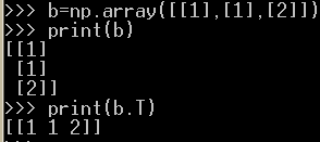
 - We use ".T" to calculate the Transposition of matrix

1 2 3 4 5 6 7 8 9 10 11 12 13 14 15

b = np.array([[1], [1], [2]]) print(b) #Transposition print(b.T) A = np.array([[1, 2, 3], [5, 4, 1], [6, 7, 4]]) #print A print(A) #Transposition print(A.T)

Figure: calculate the Transposition of matrix using numpy

3.5 Matrix Calculations

3.5.1. Addition

$A+B=\begin{bmatrix} 2 & 4\\ 2 & 5 \end{bmatrix} + \begin{bmatrix} 1 & 0\\ 3 & 1 \end{bmatrix} = \begin{bmatrix} 2+1 & 4+0\\ 2+3 & 5+1 \end{bmatrix} = \begin{bmatrix} 3 & 4\\ 5 & 6 \end{bmatrix}$ 

1 2 3 4 5 6 7 8 9 10 11

#Matrix Calculations #Addition #Commutative: A+B=B+A #Associative: (A+B)+C=A+(B+C) A = np.array([[2, 4], [2, 5]) B = np.array([[1, 0], [3, 1]) print(A) print(B) print(A+B)

Figure: Add 2 matrices

- Commutative: A+B=B+A

- Associative:  (A+B)+C=A+(B+C)
3.5.2. Subtraction

$A+B=\begin{bmatrix} 2 & 4\\ 5 & 3 \end{bmatrix} - \begin{bmatrix} 1 & 2\\ 3 & 4 \end{bmatrix} = \begin{bmatrix} 1 & 2\\ 2 & -1 \end{bmatrix}$

1 2 3 4 5 6

#Subtraction A = np.array([[2, 4], [5, 3]]) B = np.array([[1, 2], [3, 4]]) print(A) print(B) print(A-B)

 Figure: Subtract 2 matrices

3.5.3. Scalar multiplication

- Scalar x matrix = scalar multiplication

 
Figure: Scalar multiplication

1 2 3 4 5

#Scalar multiplication #Scalar x matrix = scalar multiplication A = np.array([[1, 2], [3, 4]]) print(A) print(2*A)

Figure: Scalar x matrix

3.5.4. Matrix Multiplication

A is a MxN matrix and B is a RxS matrix. AxB is possible if N=R (Number of columns in A = Number of rows in B). The result will be an MxS matrix.

 Figure: matrix A x matrix B

1 2 3 4 5 6 7

A = np.array([[1, 0], [2, 3]]) B = np.array([[2, 3], [1, 1]]) print(A) print(B) #Matrix Multiplication print(A.dot(B))

Figure: Matrix Multiplication

- Matrix multiplication is NOT commutative: AB≠BA

- Matrix multiplication IS associative: A(BC)=(AB)C
- Matrix multiplication IS distributive: A(B+C)=AB+AC and (A+B)C=AC+BC

3.6 Vector Products

Suppose that we have 2 vectors x and y

$x=\begin{bmatrix} x_{1}\\ x_{2}\\ x_{3} \end{bmatrix} y=\begin{bmatrix} y_{1}\\ y_{2}\\ y_{3} \end{bmatrix}$ 

 The vector product is calculated as below

$x^{T}y = \begin{bmatrix} x_{1} & x_{2} & x_{3} \end{bmatrix} \begin{bmatrix} y_{1}\\ y_{2}\\ y_{3} \end{bmatrix} = x_{1}y_{1} + x_{2}y_{2} + x_{3}y_{3} = \sum_{1}^{3}x_{i}y_{i}$

1 2 3 4 5 6 7

x = np.array([[1], [2], [3]]) y = np.array([[4], [5], [6]]) print(x) print(y) #Vector Products print(x.T.dot(y))

Figure:Vector Products

3.7 Identity matrix

It is similar to the number 1 in number multiplication (e.g: 1x2 = 2). It is called Identity matrix.

Figure: Identity matrix

- Matrix A is nxn , we have  A In = In A = A

- Matrix A is nxm , we have In A = A, and  A Im = A
- We use eye(size) function to create identity matrix.

1 2 3 4 5 6 7 8

#Identity matrix x = np.array([[1, 2, 3], [4, 5, 6], [7, 8, 9]]) i = np.eye(3) print(x) print(i) #Identity matrix print(x.dot(i))

Figure: Identity matrix

3.8 Matrix inverse

- A matrix A is called  invertible if there exists a matrix B such that:

- Notation for the inverse of a matrix A is A-1

- The inverse matrix is unique if it exists. And if A is invertible, then A-1 is also invertible and (AT)-1 = (A-1)T
- Matrix division: A/B= A*B-1
- In numpy we have to use this: from numpy.linalg import inv

1 2 3 4 5 6 7 8 9 10 11 12

#Matrix inverse from numpy.linalg import inv A = np.array([[1, 2], [3, 4]]) print(A) #Matrix inverse print(inv(A)) #(AT)-1 = (A-1)T print(inv(A.T)) print(inv(A).T)

Figure:Matrix inverse

3.9 Determinants

- Determinants can only be found for square matrices. 

- A matrix A has an inverse matrix A-1  if and only if det(A)≠0. Because:

 Figure: calculate A-1

- For a 2x2 matrix A, det(A) = ad-bc

Figure: Determinants for 2x2 matrix

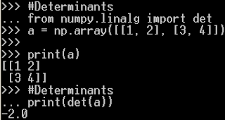
- In numpy we have to use: from numpy.linalg import det

1 2 3 4 5 6 7

#Determinants from numpy.linalg import det a = np.array([[1, 2], [3, 4]]) print(a) #Determinants print(det(a))

Figure: Determinants