Studying Keras - Convolution Neural Network

1. Concept
2. How to build Models in Keras
2 ways to build models in Keras:
- Using Sequential : different predefined layers are stacked in a stack.
- Using Functional API to build complex models.
E.g: example of using Sequential

model = Sequential()
model.add(Dense(N_HIDDEN, input_shape=(784,)))
model.add(Activation('relu'))
model.add(Dropout(DROPOUT))
model.add(Dense(N_HIDDEN))
model.add(Activation('relu'))
model.add(Dropout(DROPOUT))
model.add(Dense(nb_classes))
model.add(Activation('softmax'))
model.summary()

3. Prebuilt layers in Keras
A Dense model is a fully connected neural network layer.
RNN layers (Recurrent, SimpleRNN, GRU, LSTM)
CNN layers (Conv1D, Conv2D, MaxPooling1D, MaxPooling2D)
4. Regularization
kernel_regularizer: Regularizer function applied to the weight matrix
bias_regularizer: Regularizer function applied to the bias vector
activity_regularizer: Regularizer function applied to the output of
Dropout regularization is frequently used
Note:
+ you can write your regularizers in an object-oriented way
5. Batch normalization
It is a way to accelerate learning and generally achieve better accuracy.

1	keras.layers.normalization.BatchNormalization()

6. Activation functions

7. Losses functions
There are 4 categories:
- Accuracy : is for classification problems.
+ binary_accuracy : for binary classification problems
+ categorical_accuracy : for multiclass classification problems
+ sparse_categorical_accuracy : for sparse targets
+ top_k_categorical_accuracy : for the target class is within the top_k predictions
- Error loss : the difference between the values predicted and the values actually observed.
+ mse : mean square error
+ rmse : root square error
+ mae : mean absolute error
+ mape : mean percentage error
+ msle : mean squared logarithmic error
- Hinge loss : for training classifiers. There are two versions: hinge and squared hinge
- Class loss : to calculate the cross-entropy for classification problems:
+ binary cross-entropy
+ categorical cross-entropy
8. Metrics
A metric is a function that is used to judge the performance of your model. It is similar to an objective function but the results from evaluating a metric are not used when training the model.
9. Optimizers
Optimizers are SGD, RMSprop, and Adam.
10. Saving and loading the model

from keras.models import model_from_json 

# save as JSON 
json_string = model.to_json()
# save as YAML yaml_string = model.to_yaml()
#load model from JSON: 
model = model_from_json(json_string)

from keras.models import load_model 

#save model weights
model.save('my_model.h5')
#load model weights
model = load_model('my_model.h5')

10. Callbacks for customizing the training process
- The training process can be stopped when a metric has stopped improving by using keras.callbacks.EarlyStopping()
- You can define callback: class LossHistory(keras.callbacks.Callback)
- Check pointing saves a snapshot of the application's state at regular intervals, so the application can be restarted/recovered from the last saved state in case of failure. The state of a deep learning model is the weights of the model at that time. Using ModelCheckpoint(). Set save_best_only to true only saving a checkpoint if the current metric is better than the previously saved checkpoint.
- Using TensorBoard and Keras:

1
2
3

keras.callbacks.TensorBoard(log_dir='./logs', histogram_freq=0,write_graph=True, write_images=False)

#tensorboard --logdir=/full_path_to_your_logs

- Using Quiver and Keras : a tool for visualizing ConvNets features in an interactive way.
11. A simple neural net in Keras
11.1 Input/Output
X_train : training set
Y_train : labels of training set
We reserve apart of the training data (test set) for measuring the performance on the validation while training.
X_test : test set
Y_test : labels of test set
Data is converted into float32 for supporting GPU computation and normalized to [0, 1]
Use MNIST images, each image is a 28x28 pixels. So create a neural network with 28x28 neurons, one neuron for one pixel.
Each pixel has intensity 255, so we divide it with 255 to normalize in the range [0, 1].
The final layer only has a neuron with activation function softmax. It "squashes" a K-dimensional vector of arbitrary real values to a K-dimensional vector of real values, where each entry is in the range (0, 1). In this example, the output value is in [0-9] so K = 10.
Note: One-hot encoding - OHE
In recognizing handwritten digits, the output value is in [0-9] can be encoded into a binary vector with 10 positions, which always has 0 value, except the d-th position where a 1 is present.
11.2 Setup model
Compile (compile()) the model by selecting:
- optimizer : the specific algorithm used to update weights when training our model.
- objective function - loss function - cost function : used by the optimizer to map an event or values of one or more variables onto a real number intuitively representing some "cost" associated with the event. In this case it is to be minimized.
- metrics to evaluate the trained model
11.3 Train model
Trained with the fit()
- epoches: number of times the optimizer tries to adjust the weights so that the objective function is minimized.
- batch_size : number of samples that the optimizer performs a weight update.
- validation_split : reserve a part of the training set for validation.
Note: On Linux, we can use the command "nvidia-smi" to show GPU memory used so that you can increase batch size if not fully utilized.
Evaluate the network with evaluate() with (X_test, Y_test)

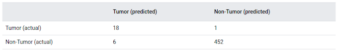
Figure: Result of training simple model

11.4 Visualize Model Training History
This helps :
- Checking convergence and over fitting when training.
- History callback is registered when training all deep learning models. It records:
+ accuracy on the training and validation datasets over training epochs.
+ loss on the training and validation datasets over training epochs.
+ Use results of history.history.keys() returns ['acc', 'loss', 'val_acc', 'val_loss']. So plot them :
plt.plot(history.history['acc'])
plt.plot(history.history['val_acc'])
plt.plot(history.history['loss'])
plt.plot(history.history['val_loss'])
11.5 Improving the simple net
Note: For every experiments we have to plot the charts to compare the effect.
- Add additional layers (hidden layers) to our network. After the first hidden layer, we add second hidden layer, again with the N_HIDDEN neurons and an activation function RELU.

1 2	model.add(Dense(N_HIDDEN)) model.add(Activation('relu'))

Figure: Add additional layers

- Using Dropout. This is a form of regularization. It randomly drop with the dropout probability some of the neurons of hidden layers. In testing phase, there is no dropout, so we are now using all our highly tuned neurons.

1
2
3

model.add(Dense(N_HIDDEN))
model.add(Activation('relu'))
model.add(Dropout(DROPOUT))

- Testing different optimizers. Keras supports stochastic gradient descent (SGD) and optimization algorithms RMSprop and Adam. RMSprop and Adam used the concept of momentum in addition to SGD. These combinations improve the accuracy and training speed.

from keras.optimizers import RMSprop, Adam
...
OPTIMIZER = RMSprop() # optimizer,
#OPTIMIZER = Adam() # optimizer

Figure: Accuracy when using Adam and RMSprop

Figure: Dropout combine Adam algorithm

- Adjusting the optimizer learning rate. This can help.

1
2
3

keras.optimizers.SGD(lr=0.01, momentum=0.0, decay=0.0, nesterov=False)
#keras.optimizers.RMSprop(lr=0.001, rho=0.9, epsilon=None, decay=0.0)
#keras.optimizers.Adam(lr=0.001, beta_1=0.9, beta_2=0.999, epsilon=None, decay=0.0, amsgrad=False)

Figure: The accuracy when changing learning rate

- Increasing the number of internal hidden neurons. The complexity of the model increases, one epoch time increases because there are more parameters to optimize. The accuracy may increase.

Figure: The accuracy when changing number of neurons

- Increasing the training batch size. Look the accuracy chart to choose the optimal batch size.

Figure: The accuracy when changing batch size

- Increasing the number of epochs

Figure: The accuracy when changing epochs, not improve

11.6 Avoiding over-fitting
Learning is more about generalization than memorization.
Look the graph below:

Figure: loss function on both validation and training sets

Loss function decreasing on both validation and training sets. However, a certain point the loss on validation starts to increase. This is over-fitting and we have a problem with model complexity.
The complexity of a model can be measured by the number of nonzero weights.
If we have 2 models M1 and M2, with the same result of loss function over training epochs, then we should choose the simplest model that has the minimum complexity.
In order to avoid over-fitting we use regularization. Keras supports both L1 (lasso, use absolute values), L2 (ridge, use square values), and elastic net (combine L1+L2) regularizations.
11.7 Summarizing the experiments
We create a summarized table:

Figure: experiments summarized table

11.8 Hyper-parameters tuning
As above, we have multiple parameters that need to be optimized. This process is Hyperparameter tuning. This process find the optimal combination of those parameters that minimize cost functions. There are some ways:
+ Grid search: build a model for each possible combination of all of the hyperparameter values provided.
E.g:
param1 = [10, 50, 100]
param2 = [3, 9, 27]
=> all possible combinations:[10,3];[10,9];[10,27];[50,3];[50,9];[50,27];[100,3];[100,9];[100,27]
+ Random search : build a statistical distribution for each hyperparameter then values may be chosen randomly. We use this in case hyperparameters have different impact.
+ Bayesian optimization : the next hyperparameters are a improvement that based on the of training result of previous hyperparameters.
Refer here.
11.9 Predicting output
Using:
predictions = model.predict(X) : compute outputs
model.evaluate() : compute the loss values
model.predict_classes() : compute category outputs
model.predict_proba() : compute class probabilities
12. Convolutional neural network (CNN)
General deep network do not care about the spatial structure and relations of each image. But convolutional neural networks (ConvNet) cares about the spatial information so it improves image classification. CNN uses convolution and pooling to do that. A ConvNet has multiple filters stacked together which learn to recognize specific visual features independently in the image.

1
2
3

model = Sequential()
model.add(Conv2D(32, (3, 3), input_shape=(256, 256, 3))
model.add(MaxPooling2D(pool_size = (2, 2)))

Applying a 3 x 3 convolution on a 256 x 256 image with three input channels and 32 filters, and max polling.
13. Simple net vs Deep CNN
Using MINST data, we test these 2 networks by reducing training set size with 5,900; 3,000; 1,800; 600 and 300. Test set size still be 10,000 examples. All the experiments are run for four training iterations.

Figure: Deep CNN is better than Simple net, even when it has more weights but less training data

13. Recognizing CIFAR-10 images with deep learning
The CIFAR-10 dataset contains 60,000 color images of 32 x 32 pixels in 3 channels divided into 10 classes. Each class contains 6,000 images. The training set size is 50,000 images, while the test sets size is 10,000 images.
The goal is to recognize unseen images and assign them to one of the 10 classes.

Figure: CIFAR-10 images

13.1 First simple deep network
13.2 Increasing the depth of network
13.3 Increasing data with data augmentation
This method generates more images for our training. We take the available CIFAR training set and augment this training set with multiple types of transformations including rotation, rescaling, horizontal/vertical flip, zooming, channel shift, ...
13.4 Extracting features from pre-built deep learning models
Each layer learns to identify the features of input that are necessary for the final classification.
Higher layers compose lower layers features to form shapes or objects.
13.5 Transfer learning
Reuse pre-trained CNNs to generate new CNN where the data set may not be large enough to train entire CNN from scratch.
to be continued ...