1. What is feature?
Consider the image:

+ Black rectangle is on edge. If we move it in vertical direction, it changes. If we move it along the edge, it looks the same.
+ Red rectangle, it is a corner. if we move it, it looks different. So it is special. And corners are considered to be good features in an image.
Feature Detection : finding regions in images which have maximum variation when moved (by a small amount) in all regions around it.
Feature Description : describe the region around the feature so that the feature can be found in other images (we can stitch them).
Note: install this package before starting. just run:
Refer to A Combined Corner and Edge Detector paper by Chris Harris & Mike Stephens
This algorithm basically finds the difference in intensity for a displacement of (u,v) in all directions.
$E(u,v)=\sum_{x,y}^{ }w(x,y)[I[x+u,y+v]-I[x,y]]^{2}$
$w(x,y)$: window function
$I[x+u,y+v]$: shifted intensity
$I[x,y]$: intensity
Then we maximize this function to find corners using Taylor Expansion and Sobel derivatives in x and y.
A score function is defined to determine if a window can contain a corner or not. Its formula:
$R=\lambda _{1}\lambda _{2}-k(\lambda _{1}+\lambda _{2})^{2}$
The result of Harris Corner Detection is a gray scale image with scores. Thresholding it to mark the corners in the image.
OpenCV provides cv2.cornerHarris(). Its arguments are :
+ img - Input image, it should be grayscale and float32 type.
+ blockSize - It is the size of neighborhood considered for corner detection
+ ksize - Aperture parameter of Sobel derivative used.
+ k - Harris detector free parameter in the equation.
Apply Harris algorithm for image below:


Shi-Tomasi score function was proposed:
$R=min(\lambda _{1},\lambda _{2})$
If it is a greater than a threshold value, it is considered as a corner.
Input image should be a gray scale image.
OpenCV has a function, cv2.goodFeaturesToTrack(). Its arguments:
+ Specify number of corners you want to find.
+ specify the quality level (between 0-1), which denotes the corner which quality is below this, will be rejected.
+ The minimum euclidean distance between corners detected.
Apply Shi-Tomasi for the image above:

4.1 Concept
As its name, this algorithm will cover the case where image is scaled.
There are 4 steps:
Step 1: Scale-space Extrema Detection
Take the original image, calculate Difference of Gaussian (DoG) of it. It is obtained as the difference of Gaussian blurring of that image with two different scales (blur levels) $\sigma$ and $k\sigma$. Then, you resize the original image to half size (create another octaves) and do the similar process. As the figure below:


This step eliminates any low-contrast keypoints and edge keypoints.
In order to eliminate potential keypoints, Taylor series expansion was used to calculate an intensity. If the intensity at this extrema is less than a threshold value, it is rejected. This threshold is called contrastThreshold in OpenCV.
In order to eliminate edges, 2x2 Hessian matrix was used to calculate a ratio. If this ratio is greater than a threshold, called edgeThreshold in OpenCV.
Step 3: Orientation Assignment
Assigned orientation to each keypoint to achieve invariance to image rotation.
The magnitude and orientation is calculated for all pixels around the keypoint. An orientation histogram with 36 bins covering 360 degrees is created. The highest peak and peaks above 80% of it in the histogram are considered to calculate the orientation. It creates keypoints with same location and scale, but different orientations.
Step 4: Keypoint Descriptor
Take a 16x16 neighborhood around the keypoint and devide it into 16 sub-blocks of 4x4 size. For each sub-block, 8 bin orientation histogram is created. So a total of 128 bin values are available. It is represented as a vector to form keypoint descriptor.
Step 5: Keypoint Matching
Keypoints between two images are matched by identifying their nearest neighbours.
4.2 SIFT in OpenCV
First we have to construct a SIFT object "sift"
sift.detect() function finds the keypoint in the images.
cv2.drawKeyPoints() draws the small circles on the location and orientation of keypoints.
sift.compute() which computes the descriptors from the keypoints
sift.detectAndCompute() find keypoints and descriptors in one step.
Apply SIFT for the image above:

5.1 Concept
SURF is 3 times faster than SIFT. SURF is good at handling images with blurring and rotation, but not good at handling viewpoint change and illumination change.
Instead of using DoG, SURF approximates LoG with Box Filter.
For orientation assignment, SURF uses wavelet responses in horizontal and vertical direction for a neighborhood of size 6s. In case rotation invariance is not required, Upright-SURF or U-SURF (upright flag in OpenCV) is used to speed up the process.
For feature description, SURF uses Wavelet responses in horizontal and vertical direction.
SURF feature descriptor has 64 dimensions and extended 128 dimension version. OpenCV supports both by setting the value of flag extended with 0 and 1 for 64-dim and 128-dim.
It uses sign of Laplacian to distinguishe bright blobs on dark backgrounds from the reverse situation. So in the matching step, only features that have the same type of contrast, will be compared, as image below:
 Refer to SURF: Speeded Up Robust Features paper.
5.2 SURF in OpenCV
Apply SURF for image below:


It is several times faster than other existing corner detectors.
It is not robust to high levels of noise.
It depends on a threshold.
Refer to Machine learning for high-speed corner detection.
The algorithm:
+ Select a test pixel p in the image and its intensity be Ip.
+ Select threshold value t.
+ Consider a circle of 16 pixels around the test pixel.
 + The pixel p is a corner if there are n contiguous pixels in the circle (white dash lines of 16 pixels) which are all brighter than Ip+t, or all darker than Ip−t.. n was chosen to be 12.
+ A high-speed test examines only the four pixels at 1, 9, 5 and 13. If p is a corner, then at least three of these must all be brighter than Ip+t or darker than Ip−t.
+ The full segment test examines all pixels in the circle.
+ There are several weaknesses:
++ It does not reject as many candidates for n < 12.
++ The choice of pixels is not optimal because its efficiency depends on ordering of the questions and distribution of corner appearances.
++ Results of high-speed tests are thrown away.
++ Multiple features are detected adjacent to one another.
First 3 points are addressed with a machine learning approach. Last one is addressed using non-maximal suppression.
6.2 FAST in OpenCV
Arguments:
+ Specify the threshold
+ non-maximum suppression to be applied or not.
+ the neighborhood, three flags are defined, cv.FAST_FEATURE_DETECTOR_TYPE_5_8, cv.FAST_FEATURE_DETECTOR_TYPE_7_12 and cv.FAST_FEATURE_DETECTOR_TYPE_9_16.
Apply FAST for image:


7.1 Concept
BRIEF is a faster method feature descriptor calculation and matching. It also provides high recognition rate if there is not large in-plane rotation.
A vector with thousands of features consumes a lot of memory. Moreover, larger the memory, longer the time it takes for matching. These are not feasible for the low resource systems. So we need to compress it using methods such as PCA, LDA, LSH (Locality Sensitive Hashing).
LSH converts SIFT descriptors from floating point numbers to binary strings. These binary strings are used to match features using Hamming distance.
BRIEF finds the binary strings directly without finding descriptors.
Refer to Binary Robust Independent Elementary Features paper.
From smoothed image, BRIEF takes $n_{d}(x,y)$ pairs. For each pair, compare the intensity of 2 pixels, if $I(p)<I(q)$ result is 1, else it is 0. Repeat for $n_{d}(x,y)$ pairs.
$n_{d}(x,y)$ can be 128, 256, 512. OpenCV represents it in bytes so the values will be 16, 32 and 64. Then using Hamming Distance to match these descriptors.
The paper recommends to use CenSurE to find the features and then apply BRIEF.
7.2 BRIEF in OpenCV
Apply FAST+BRIEF for the image above:

Refer to ORB: An efficient alternative to SIFT or SURF paper.
ORB is an improvement of FAST keypoint detector and BRIEF descriptor. it implement many modifications to enhance the performance.
OpenCV provides cv2.ORB() or using feature2d common interface, with main arguments:
+ nFeatures : maximum number of features to be retained (by default 500)
+ scoreType : Harris score or FAST score to rank the features (by default, Harris score)
+ WTA_K : number of points that produce each element of the oriented BRIEF descriptor.
++ WTA_K=2, NORM_HAMMING distance is used for matching
++ WTA_K=3 or 4, NORM_HAMMING2 distance is used for matching
Apply ORB for image above:

It takes the descriptor of one feature in first set and compare with all features in second set using specific distance calculation. And the closest one is returned.
OpenCV creates BFMatcher object using cv2.BFMatcher() with 2 optinal arguments:
+ normType : specify the distance measurement to be used.
++ cv2.NORM_L2 (default value) is for SIFT, SURF
++ cv2.NORM_HAMMING is for binary string based descriptors like ORB, BRIEF, BRISK
++ cv2.NORM_HAMMING2 is for ORB is using WTA_K == 3 or 4
+ crossCheck : the two features in both sets should match each other. The matched result with value (i,j) such that i-th descriptor in set A has j-th descriptor in set B as the best match and vice-versa.
+ BFMatcher.match() : returns the best match
+ BFMatcher.knnMatch() : returns k best matches
+ cv2.drawMatches() : draws the matches
+ cv2.drawMatchesKnn : draws all the k best matches
The DMatch object has following attributes:
+ DMatch.distance - Distance between descriptors. The lower, the better it is.
+ DMatch.trainIdx - Index of the descriptor in train descriptors
+ DMatch.queryIdx - Index of the descriptor in query descriptors
+ DMatch.imgIdx - Index of the train image.
Apply Matching with SIFT Descriptors for the image below:


How to find the object exactly on the source image?
We pass a set of points from both the images to cv2.findHomography() to find the perspective transformation of that object (It needs at least four points to find the transformation). Using RANSAC or LEAST_MEDIAN algorithm flag to eliminate abnormal data.
Then we use cv2.perspectiveTransform() to find the object.
Reuse the example above:

Consider the image:
Figure: example of feature (from OpenCV)
+ Blue rectangle is flat area. If we move the blue rectangle, it looks the same. So it is not special.+ Black rectangle is on edge. If we move it in vertical direction, it changes. If we move it along the edge, it looks the same.
+ Red rectangle, it is a corner. if we move it, it looks different. So it is special. And corners are considered to be good features in an image.
Feature Detection : finding regions in images which have maximum variation when moved (by a small amount) in all regions around it.
Feature Description : describe the region around the feature so that the feature can be found in other images (we can stitch them).
Note: install this package before starting. just run:
pip install opencv-contrib-python
2. Harris Corner DetectionRefer to A Combined Corner and Edge Detector paper by Chris Harris & Mike Stephens
This algorithm basically finds the difference in intensity for a displacement of (u,v) in all directions.
$E(u,v)=\sum_{x,y}^{ }w(x,y)[I[x+u,y+v]-I[x,y]]^{2}$
$w(x,y)$: window function
$I[x+u,y+v]$: shifted intensity
$I[x,y]$: intensity
Then we maximize this function to find corners using Taylor Expansion and Sobel derivatives in x and y.
A score function is defined to determine if a window can contain a corner or not. Its formula:
$R=\lambda _{1}\lambda _{2}-k(\lambda _{1}+\lambda _{2})^{2}$
The result of Harris Corner Detection is a gray scale image with scores. Thresholding it to mark the corners in the image.
OpenCV provides cv2.cornerHarris(). Its arguments are :
+ img - Input image, it should be grayscale and float32 type.
+ blockSize - It is the size of neighborhood considered for corner detection
+ ksize - Aperture parameter of Sobel derivative used.
+ k - Harris detector free parameter in the equation.
Apply Harris algorithm for image below:

Figure: input image to apply Harris
1 2 3 4 5 6 7 8 9 10 11 12 13 14 15 16 | import cv2 import numpy as np filename = 'images/wall.png' img = cv2.imread(filename) gray = cv2.cvtColor(img,cv2.COLOR_BGR2GRAY) gray = np.float32(gray) dst = cv2.cornerHarris(gray,3,9,0.04) # Threshold for an optimal value, it may vary depending on the image. img[dst>0.1*dst.max()]=[0,0,255] cv2.imshow('dst',img) cv2.waitKey(0) cv2.destroyAllWindows() |

Figure: adjusting arguments to achieve good result
3. Shi-Tomasi Corner Detector & Good Features to Track Shi-Tomasi score function was proposed:
$R=min(\lambda _{1},\lambda _{2})$
If it is a greater than a threshold value, it is considered as a corner.
Input image should be a gray scale image.
OpenCV has a function, cv2.goodFeaturesToTrack(). Its arguments:
+ Specify number of corners you want to find.
+ specify the quality level (between 0-1), which denotes the corner which quality is below this, will be rejected.
+ The minimum euclidean distance between corners detected.
Apply Shi-Tomasi for the image above:
1 2 3 4 5 6 7 8 9 10 11 12 13 14 15 | import numpy as np import cv2 img = cv2.imread('images/wall.png') gray = cv2.cvtColor(img,cv2.COLOR_BGR2GRAY) corners = cv2.goodFeaturesToTrack(gray,500,0.3,4) for i in corners: x,y = i.ravel() cv2.circle(img,(x,y),2, (0,0,255),-1) cv2.imshow('dst',img) cv2.waitKey(0) cv2.destroyAllWindows() |

Figure: adjusting arguments to achieve good result
4. Scale-Invariant Feature Transform (SIFT)4.1 Concept
As its name, this algorithm will cover the case where image is scaled.
There are 4 steps:
Step 1: Scale-space Extrema Detection
Take the original image, calculate Difference of Gaussian (DoG) of it. It is obtained as the difference of Gaussian blurring of that image with two different scales (blur levels) $\sigma$ and $k\sigma$. Then, you resize the original image to half size (create another octaves) and do the similar process. As the figure below:
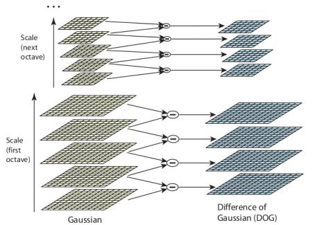
Figure: calculate DoG for octaves
Search for local maxima/minima in DoG images by taking one pixel in DoG image and compare with its 8 neighbours as well as 9
pixels in next scale and 9 pixels in previous scales. If it is a local
extrema, it is a potential keypoint.
Figure: Search for local maxima/minima in DoG images
Step 2: Keypoint Localization This step eliminates any low-contrast keypoints and edge keypoints.
In order to eliminate potential keypoints, Taylor series expansion was used to calculate an intensity. If the intensity at this extrema is less than a threshold value, it is rejected. This threshold is called contrastThreshold in OpenCV.
In order to eliminate edges, 2x2 Hessian matrix was used to calculate a ratio. If this ratio is greater than a threshold, called edgeThreshold in OpenCV.
Step 3: Orientation Assignment
Assigned orientation to each keypoint to achieve invariance to image rotation.
The magnitude and orientation is calculated for all pixels around the keypoint. An orientation histogram with 36 bins covering 360 degrees is created. The highest peak and peaks above 80% of it in the histogram are considered to calculate the orientation. It creates keypoints with same location and scale, but different orientations.
Step 4: Keypoint Descriptor
Take a 16x16 neighborhood around the keypoint and devide it into 16 sub-blocks of 4x4 size. For each sub-block, 8 bin orientation histogram is created. So a total of 128 bin values are available. It is represented as a vector to form keypoint descriptor.
Step 5: Keypoint Matching
Keypoints between two images are matched by identifying their nearest neighbours.
4.2 SIFT in OpenCV
First we have to construct a SIFT object "sift"
sift.detect() function finds the keypoint in the images.
cv2.drawKeyPoints() draws the small circles on the location and orientation of keypoints.
sift.compute() which computes the descriptors from the keypoints
sift.detectAndCompute() find keypoints and descriptors in one step.
Apply SIFT for the image above:
1 2 3 4 5 6 7 8 9 10 11 12 13 14 | import cv2 import numpy as np img = cv2.imread('wall.png') gray= cv2.cvtColor(img,cv2.COLOR_BGR2GRAY) sift = cv2.xfeatures2d.SIFT_create(0,3,0.07,10,1.6) kp = sift.detect(gray,None) cv2.drawKeypoints(gray,kp,img,flags=cv2.DRAW_MATCHES_FLAGS_DRAW_RICH_KEYPOINTS) cv2.imshow('SIFT',img) cv2.waitKey(0) cv2.destroyAllWindows() |

Figure: output of SIFT
5. Speeded-Up Robust Features (SURF)5.1 Concept
SURF is 3 times faster than SIFT. SURF is good at handling images with blurring and rotation, but not good at handling viewpoint change and illumination change.
Instead of using DoG, SURF approximates LoG with Box Filter.
For orientation assignment, SURF uses wavelet responses in horizontal and vertical direction for a neighborhood of size 6s. In case rotation invariance is not required, Upright-SURF or U-SURF (upright flag in OpenCV) is used to speed up the process.
For feature description, SURF uses Wavelet responses in horizontal and vertical direction.
SURF feature descriptor has 64 dimensions and extended 128 dimension version. OpenCV supports both by setting the value of flag extended with 0 and 1 for 64-dim and 128-dim.
It uses sign of Laplacian to distinguishe bright blobs on dark backgrounds from the reverse situation. So in the matching step, only features that have the same type of contrast, will be compared, as image below:

5.2 SURF in OpenCV
Apply SURF for image below:

Figure: input image for SURF
1 2 3 4 5 6 7 8 9 10 11 12 13 14 15 | import cv2 import numpy as np img = cv2.imread('surf.png') gray= cv2.cvtColor(img,cv2.COLOR_BGR2GRAY) #here the Hessian threshold is 20000 surf = cv2.xfeatures2d.SURF_create(20000) #detect keypoints kp, des = surf.detectAndCompute(img,None) img2 = cv2.drawKeypoints(img,kp,None,(255,0,0),4) cv2.imshow('SURF',img2) cv2.waitKey(0) cv2.destroyAllWindows() |

Figure: adjusting arguments to achieve good result, and SURF act as a blobs detection (detect white objects in black background)
If Upright is enabled. We just add surf.setUpright(True)
Figure: All the orientations are shown in same direction
If using 128 dimensions version, just using surf.extended = True
6. Features from Accelerated Segment Test (FAST)
6.1 ConceptIt is several times faster than other existing corner detectors.
It is not robust to high levels of noise.
It depends on a threshold.
Refer to Machine learning for high-speed corner detection.
The algorithm:
+ Select a test pixel p in the image and its intensity be Ip.
+ Select threshold value t.
+ Consider a circle of 16 pixels around the test pixel.

+ A high-speed test examines only the four pixels at 1, 9, 5 and 13. If p is a corner, then at least three of these must all be brighter than Ip+t or darker than Ip−t.
+ The full segment test examines all pixels in the circle.
+ There are several weaknesses:
++ It does not reject as many candidates for n < 12.
++ The choice of pixels is not optimal because its efficiency depends on ordering of the questions and distribution of corner appearances.
++ Results of high-speed tests are thrown away.
++ Multiple features are detected adjacent to one another.
First 3 points are addressed with a machine learning approach. Last one is addressed using non-maximal suppression.
6.2 FAST in OpenCV
Arguments:
+ Specify the threshold
+ non-maximum suppression to be applied or not.
+ the neighborhood, three flags are defined, cv.FAST_FEATURE_DETECTOR_TYPE_5_8, cv.FAST_FEATURE_DETECTOR_TYPE_7_12 and cv.FAST_FEATURE_DETECTOR_TYPE_9_16.
Apply FAST for image:
Figure: input image for FAST
1 2 3 4 5 6 7 8 9 10 11 12 13 14 15 16 17 18 19 20 21 22 | import numpy as np import cv2 as cv img = cv.imread('images/wall.png') gray= cv.cvtColor(img,cv.COLOR_BGR2GRAY) # Initiate FAST object with default values fast = cv.FastFeatureDetector_create(55,True,cv.FAST_FEATURE_DETECTOR_TYPE_9_16 ) # find and draw the keypoints kp = fast.detect(gray,None) img2 = cv.drawKeypoints(img, kp, None, color=(255,0,0)) # Print all default params print( "Threshold: {}".format(fast.getThreshold()) ) print( "nonmaxSuppression:{}".format(fast.getNonmaxSuppression()) ) print( "neighborhood: {}".format(fast.getType()) ) print( "Total Keypoints with nonmaxSuppression: {}".format(len(kp)) ) cv.imwrite('fast_true.png',img2) # Disable nonmaxSuppression fast.setNonmaxSuppression(0) kp = fast.detect(img,None) print( "Total Keypoints without nonmaxSuppression: {}".format(len(kp)) ) img3 = cv.drawKeypoints(img, kp, None, color=(255,0,0)) cv.imwrite('fast_false.png',img3) |

Figure: no apply non-maximum suppression+adjusting threshold

Figure: apply non-maximum suppression+adjusting threshold
7. Binary Robust Independent Elementary Features (BRIEF)7.1 Concept
BRIEF is a faster method feature descriptor calculation and matching. It also provides high recognition rate if there is not large in-plane rotation.
A vector with thousands of features consumes a lot of memory. Moreover, larger the memory, longer the time it takes for matching. These are not feasible for the low resource systems. So we need to compress it using methods such as PCA, LDA, LSH (Locality Sensitive Hashing).
LSH converts SIFT descriptors from floating point numbers to binary strings. These binary strings are used to match features using Hamming distance.
BRIEF finds the binary strings directly without finding descriptors.
Refer to Binary Robust Independent Elementary Features paper.
From smoothed image, BRIEF takes $n_{d}(x,y)$ pairs. For each pair, compare the intensity of 2 pixels, if $I(p)<I(q)$ result is 1, else it is 0. Repeat for $n_{d}(x,y)$ pairs.
$n_{d}(x,y)$ can be 128, 256, 512. OpenCV represents it in bytes so the values will be 16, 32 and 64. Then using Hamming Distance to match these descriptors.
The paper recommends to use CenSurE to find the features and then apply BRIEF.
7.2 BRIEF in OpenCV
Apply FAST+BRIEF for the image above:
1 2 3 4 5 6 7 8 9 10 11 12 13 14 15 16 | import numpy as np import cv2 as cv img = cv.imread('wall.png') gray= cv.cvtColor(img,cv.COLOR_BGR2GRAY) # Initiate FAST object with default values fast = cv.FastFeatureDetector_create(55,True,cv.FAST_FEATURE_DETECTOR_TYPE_9_16 ) # Initiate BRIEF extractor brief = cv.xfeatures2d.BriefDescriptorExtractor_create(64, True) # find and draw the keypoints kp = fast.detect(gray,None) # compute the descriptors with BRIEF kp, des = brief.compute(gray, kp) print brief.descriptorSize() img2 = cv.drawKeypoints(img, kp, None, color=(255,0,0)) cv.imwrite('fast_true.png',img2) |

Figure: after applying BRIEF, comparing to previouys result
8. Oriented FAST and Rotated BRIEF (ORB) Refer to ORB: An efficient alternative to SIFT or SURF paper.
ORB is an improvement of FAST keypoint detector and BRIEF descriptor. it implement many modifications to enhance the performance.
OpenCV provides cv2.ORB() or using feature2d common interface, with main arguments:
+ nFeatures : maximum number of features to be retained (by default 500)
+ scoreType : Harris score or FAST score to rank the features (by default, Harris score)
+ WTA_K : number of points that produce each element of the oriented BRIEF descriptor.
++ WTA_K=2, NORM_HAMMING distance is used for matching
++ WTA_K=3 or 4, NORM_HAMMING2 distance is used for matching
Apply ORB for image above:
1 2 3 4 5 6 7 8 9 10 11 12 13 14 15 16 17 18 | import cv2 import numpy as np img = cv2.imread('wall.png') gray= cv2.cvtColor(img,cv2.COLOR_BGR2GRAY) # Initiate ORB detector orb = cv2.ORB_create(300,1.1,4,10,0,2,1,31,10) # find the keypoints with ORB kp = orb.detect(img,None) # compute the descriptors with ORB kp, des = orb.compute(img, kp) # draw only keypoints location,not size and orientation img2 = cv2.drawKeypoints(img, kp, None, color=(255,0,0), flags=0) cv2.imshow('ORB',img2) cv2.waitKey(0) cv2.destroyAllWindows() |

Figure: output of ORB
9. Feature MatchingIt takes the descriptor of one feature in first set and compare with all features in second set using specific distance calculation. And the closest one is returned.
OpenCV creates BFMatcher object using cv2.BFMatcher() with 2 optinal arguments:
+ normType : specify the distance measurement to be used.
++ cv2.NORM_L2 (default value) is for SIFT, SURF
++ cv2.NORM_HAMMING is for binary string based descriptors like ORB, BRIEF, BRISK
++ cv2.NORM_HAMMING2 is for ORB is using WTA_K == 3 or 4
+ crossCheck : the two features in both sets should match each other. The matched result with value (i,j) such that i-th descriptor in set A has j-th descriptor in set B as the best match and vice-versa.
+ BFMatcher.match() : returns the best match
+ BFMatcher.knnMatch() : returns k best matches
+ cv2.drawMatches() : draws the matches
+ cv2.drawMatchesKnn : draws all the k best matches
The DMatch object has following attributes:
+ DMatch.distance - Distance between descriptors. The lower, the better it is.
+ DMatch.trainIdx - Index of the descriptor in train descriptors
+ DMatch.queryIdx - Index of the descriptor in query descriptors
+ DMatch.imgIdx - Index of the train image.
Apply Matching with SIFT Descriptors for the image below:

Figure: image to search
Figure: this query image was cut + rotate + scale from original image
1 2 3 4 5 6 7 8 9 10 11 12 13 14 15 16 17 18 19 20 21 22 23 24 25 | import numpy as np import cv2 from matplotlib import pyplot as plt img1 = cv2.imread('query.png') # queryImage img2 = cv2.imread('toy-story.jpg') # trainImage gray1= cv2.cvtColor(img1,cv2.COLOR_BGR2GRAY) gray2= cv2.cvtColor(img2,cv2.COLOR_BGR2GRAY) # Initiate SIFT detector sift = cv2.xfeatures2d.SIFT_create() # find the keypoints and descriptors with SIFT kp1, des1 = sift.detectAndCompute(gray1,None) kp2, des2 = sift.detectAndCompute(gray2,None) # BFMatcher with default params bf = cv2.BFMatcher() matches = bf.knnMatch(des1,des2, k=2) # Apply ratio test good = [] for m,n in matches: if m.distance < 0.5*n.distance: good.append([m]) img3 = None # cv2.drawMatchesKnn expects list of lists as matches. img3 = cv2.drawMatchesKnn(img1,kp1,img2,kp2,good,img3,flags=2) plt.imshow(cv2.cvtColor(img3, cv2.COLOR_BGR2RGB)),plt.show() |

Figure: Matching with SIFT Descriptors
10. Feature Matching + Homography to find ObjectsHow to find the object exactly on the source image?
We pass a set of points from both the images to cv2.findHomography() to find the perspective transformation of that object (It needs at least four points to find the transformation). Using RANSAC or LEAST_MEDIAN algorithm flag to eliminate abnormal data.
Then we use cv2.perspectiveTransform() to find the object.
Reuse the example above:
1 2 3 4 5 6 7 8 9 10 11 12 13 14 15 16 17 18 19 20 21 22 23 24 25 26 27 28 29 30 31 32 33 34 35 36 37 38 39 40 41 42 43 44 45 | import numpy as np import cv2 from matplotlib import pyplot as plt MIN_MATCH_COUNT = 10 img1 = cv2.imread('query.png') # queryImage img2 = cv2.imread('toy-story.jpg') # trainImage gray1= cv2.cvtColor(img1,cv2.COLOR_BGR2GRAY) gray2= cv2.cvtColor(img2,cv2.COLOR_BGR2GRAY) # Initiate SIFT detector sift = cv2.xfeatures2d.SIFT_create() # find the keypoints and descriptors with SIFT kp1, des1 = sift.detectAndCompute(gray1,None) kp2, des2 = sift.detectAndCompute(gray2,None) # BFMatcher with default params bf = cv2.BFMatcher() matches = bf.knnMatch(des1,des2, k=2) # Apply ratio test good = [] for m,n in matches: if m.distance < 0.5*n.distance: good.append([m]) if len(good)>MIN_MATCH_COUNT: src_pts = np.float32([ kp1[m[0].queryIdx].pt for m in good ]).reshape(-1,1,2) dst_pts = np.float32([ kp2[m[0].trainIdx].pt for m in good ]).reshape(-1,1,2) M, mask = cv2.findHomography(src_pts, dst_pts, cv2.RANSAC,5.0) #extract found ROI matchesMask = mask.ravel().tolist() h,w,d = img1.shape pts = np.float32([ [0,0],[0,h-1],[w-1,h-1],[w-1,0] ]).reshape(-1,1,2) dst = cv2.perspectiveTransform(pts,M) #draw rectangle img2 = cv2.polylines(img2,[np.int32(dst)],True,255,3, cv2.LINE_AA) else: print "Not enough matches are found - %d/%d" % (len(good),MIN_MATCH_COUNT) matchesMask = None draw_params = dict(matchColor = (0,255,0), # draw matches in green color singlePointColor = None, matchesMask = matchesMask, # draw only inliers flags = 2) img3 = None # cv2.drawMatchesKnn expects list of lists as matches. img3 = cv2.drawMatchesKnn(img1,kp1,img2,kp2,good,img3,flags=2) plt.imshow(cv2.cvtColor(img3, cv2.COLOR_BGR2RGB)),plt.show() |

Figure: Feature Matching + Homography to find Objects


0 Comments