Decision Trees and Random Forests

Review the example: build a decision tree to classify an animal.

How the decision tree splits the data (training)?

1. Metrics for training decision trees

1.1. Information Gain

• We want to determine which attribute in a given set of training feature vectors is most useful for discriminating between the classes to be learned (larger Information Gain).

• Information gain tells us how important a given attribute of the feature vectors is.

• We will use it to decide the ordering of attributes in the nodes of a decision tree.

Information Gain = entropy(parent) – [average entropy(children)]

1.2 Gini Impurity

Gini Impurity measures the probability of incorrect classification an observation.

GI = 1 - G

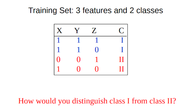
Reuse example above:

Split on Z: G = 0.5 * (1-0.5) + 0.5 *(1-0.5) = 0.5 => WORST

Split on Y: G = 1* (1-1) + 1 *(1-1) = 0

Split on X: G = 2/3* (1-2/3) + 1 *(1-1) = 2/9

Gini impurity doesn't require to compute logarithmic functions, which are computationally intensive.

2. Decision tree

2.1 Creating a decision tree

from sklearn.datasets import make_blobs
from sklearn.tree import DecisionTreeClassifier
import numpy as np
import matplotlib.pyplot as plt
import seaborn as sns
sns.set()

X, y = make_blobs(n_samples=300, centers=4, random_state=0, cluster_std=1.0)
plt.scatter(X[:, 0], X[:, 1], c=y, s=50, cmap='rainbow')
ax = plt.gca()
xlim = ax.get_xlim()
ylim = ax.get_ylim()
model = DecisionTreeClassifier()
model.fit(X, y)
nx = np.linspace(xlim[0], xlim[1], num=200)
ny = np.linspace(ylim[0], ylim[1], num=200)
xx, yy = np.meshgrid(nx, ny)
Z = model.predict(np.c_[xx.ravel(), yy.ravel()]).reshape(xx.shape)
n_classes = len(np.unique(y))
contours = ax.contourf(xx, yy, Z, alpha=0.3, levels=np.arange(n_classes + 1) - 0.5, cmap='RdBu', clim=(y.min(), y.max()), zorder=1)
ax.set(xlim=xlim, ylim=ylim)
plt.show()

2.2 Decision trees and overfitting

It is very easy to go too deep in the tree, and thus to fit details of the particular data rather than the overall properties of the distributions they are drawn from.

Overfitting can be seen by looking at models trained on different subsets of the data.

From the figure, in four corners the trees produce consistent results but in the regions between any two clusters the trees give different results (the classification is less certain). We have idea that using results from many trees would improve our results.

3. Ensembles of Decision Trees

3.1 Random Forests

The idea is using multiple overfitting estimators can be combined to reduce the effect of overfitting. This method called bagging. It uses an ensemble of parallel estimators. Each of which overfits the data, and averages the results to find a better classification.

There are bagging methods to reduce the variance of a base estimator. The difference is by the way they draw random subsets of the training set.

- When random subsets of the dataset are drawn as random subsets of the samples, then this algorithm is known as Pasting.

- When samples are drawn with replacement, then the method is known as Bagging.

- When random subsets of the dataset are drawn as random subsets of the features, then the method is known as Random Subspaces.

- When base estimators are built on subsets of both samples and features, then the method is known as Random Patches.

Ensemble of decision trees is known as a random forest.

from sklearn.datasets import make_blobs
from sklearn.tree import DecisionTreeClassifier
import numpy as np
import matplotlib.pyplot as plt
import seaborn as sns
sns.set()
from sklearn.ensemble import RandomForestClassifier
from sklearn.ensemble import BaggingClassifier

X, y = make_blobs(n_samples=300, centers=4, random_state=0, cluster_std=1.0)
plt.scatter(X[:, 0], X[:, 1], c=y, s=50, cmap='rainbow')
ax = plt.gca()
xlim = ax.get_xlim()
ylim = ax.get_ylim()

tree = DecisionTreeClassifier()
model = BaggingClassifier(tree, n_estimators=100, max_samples=0.8, random_state=1)
model.fit(X, y)
nx = np.linspace(xlim[0], xlim[1], num=200)
ny = np.linspace(ylim[0], ylim[1], num=200)
xx, yy = np.meshgrid(nx, ny)
Z = model.predict(np.c_[xx.ravel(), yy.ravel()]).reshape(xx.shape)
n_classes = len(np.unique(y))
contours = ax.contourf(xx, yy, Z, alpha=0.3, levels=np.arange(n_classes + 1) - 0.5, cmap='RdBu', clim=(y.min(), y.max()), zorder=1)
ax.set(xlim=xlim, ylim=ylim)
plt.show()

3.2 Random Forest Regression

Random Forest can be used for regression (continuous data)

import numpy as np
import matplotlib.pyplot as plt
from sklearn.ensemble import RandomForestRegressor

rng = np.random.RandomState(1)
x = 10 * rng.rand(50)
y = np.sin(x) + 0.1 * rng.randn(50)
plt.scatter(x, y)

model = RandomForestRegressor(n_estimators=100, random_state=2)
model.fit(x[:, np.newaxis], y)
xfit = np.linspace(0, 10, 1000)
predicted = model.predict(xfit[:, np.newaxis])
plt.plot(xfit, predicted, '-r')

plt.xlim(0, 10);
plt.show()