1. Introduction
2. Linear regression
3. Optimize linear regression cost function
3.1 Gradient descent
3.2 Normal Equations
4. Polynomial regression
5. Feature scaling
6. Underfitting - Overfitting
6.1 Model selection
6.2 Regularization
1. Introduction
This note focuses on Supervised learning that using Linear regression model and Gradient descent algorithm to build the linear regression model.
Note: python, numpy, basic linear algebra, matplotlib are required. Please refer to this post and this post.
Notation:

2. Linear regression
In linear regression, we use h(x) as a linear function of x to predict y. So h(x) has the form:
$h(x) = \theta _{0}x_{0} + \theta _{1}x_{1} + \theta _{2}x_{2}\\
\theta _{i}: \text{parameters or weights}\\
\text{ choose} x_{0} = 1 => h(x) = \theta _{0} + \theta _{1}x_{1} + \theta _{2}x_{2}\\
\text{or } h(x) = \sum_{1}^{n}\theta _{i}x_{i} = \theta ^{T}x\\
\theta ^{T}: \text{ is the transpose of vector }\theta\\
\theta = \begin{bmatrix} \theta _{0}\\
\theta _{1}\\ ...\\
\theta _{n} \end{bmatrix}; x = \begin{bmatrix} x_{0}\\ x_{1}\\ ...\\ x_{n} \end{bmatrix}$
The learning process is to find/learn the parameters θi to make h(x) close to y for the training examples. In order to measure how close the h(x(i)) is to the corresponding y(i) for each value of θ, we define the cost function:
3. Optimize linear regression cost function
3.1 Gradient descent
This is one of the algorithms that supports to find/learn θi to minimize J(θ). This algorithm starts with some initial of θ and repeatedly performs the update with LMS (least mean squares) or Widrow-Hoff learning rule:
$\theta _{j} = \theta _{j} - \frac{1}{m}\alpha \sum_{1}^{m}(h(x^{(i)}) - y^{(i)})x_{j}^{i} \mathbf{(1)}\\
\text{The algorithm repeats for every j until convergence \{}\\
\text{ }\theta _{j} = \theta _{j} - \frac{1}{m}\alpha \sum_{1}^{m}(h(x^{(i)}) - y^{(i)})x_{j}^{i} \mathbf{(2)}\\
\text{\}}\\
\text{The algorithm repeats for every j until convergence \{}\\
\text{ for i=1 to m \{}\\
\text{ }\theta _{j} = \theta _{j} - \frac{1}{m}\alpha (h(x^{(i)}) - y^{(i)})x_{j}^{i} \mathbf{(3)}\\
\text{ \}}\\
\text{\}}$
Formula (1): the partial derivative represents the direction to find/learn θ that can minimize J(θ).
Formula (2): on every step we update θj based on entire training examples. So it is called batch gradient descent.
Formula (3): on every step we update θj based on each training example. With this algorithm, we need not to calculate sum of all training examples that need much memory and time. It is called stochastic gradient descent or incremental gradient descent. Often, stochastic gradient descent gets θ "close" to the minimum much faster than batch gradient descent. However it may never "converge" to the minimum, and the parameters θ will keep oscillating around the minimum of J(θ); but in practice most of the values near the minimum will be reasonably good approximations to the true minimum.
- J is a convex quadratic function. So the optimization problem has only one global and gradient descent always converges.
- The learning rate determines how fast or slow the optimizer will move towards the optimal weights. You can try it here (it is λ).

Try to choose α with range [ ..., 0.001, 0.003, 0.01, 0.03, 0.1, 0.3, 1, ...] and choose the largest possible value or slightly smaller than the largest possible value.
So it is time to practise. We will make a simple demo for this algorithm. Our input only has 1 feature and 1 output. The input is a list x= [0, 0.5, 1, 1.5, ..., 9.5, 10] and output is a list y = [3, 3.5, 4, 4.5, ..., 12.5, 13] (output is generated by formula y=x+3). Applying linear regression model (y = θ0x0 + θ1x1) and gradient descent. Since we generate training set using function (y=x+3) so after training the right result will approximates to(θ0 = 3 and θ1 = 1).
Note: if your PC is not strong then disable update_line() function because it take time to plot J while calculating so the algorithm will be slow.
Here is the Python source code using batch gradient descent:


Instead of using gradient descent, we can find the optimization point of cost function directly by solving the equation:
$\frac{\delta J(\theta )}{\delta \theta } = 0\\
\text{solve it we have normal equation: }\theta = (X^{T}X)^{-1}X^{T}Y$
$\text{we have training example (i) with n features:}\\
x^{(i)} = \begin{bmatrix}
x_{0}\\
x_{1}\\
...\\
x_{n}
\end{bmatrix}
\text{then } X = \begin{bmatrix}
(x^{(1)})^{T}\\
(x^{(2)})^{T}\\
...\\
(x^{(m)})^{T}
\end{bmatrix} \in R^{mx(n+1))}\\\\
\text{and } Y = \begin{bmatrix}
y^{(1)}\\
y^{(2)}\\
...\\
y^{(m)}
\end{bmatrix}$
In case the matrix $(X^{T}X)^{-1}$ is invert-able or singular:
+ we check and remove redundant features (linear dependent features). E.g we have feature X but we also have feature $2X$. We only need X so remove $2X$.
+ if training set size m < number of features n, we consider to remove redundant features.
+ Consider using the (Moore-Penrose) pseudo-inverse of a matrix.
Using normal equation we need not care about feature scaling (discuss later).
Let 's make a demo using normal equation. We re-use demo in 3.1 the result should be theta0=3 and theta1=1
One step to the target
4. Polynomial regression
Suppose that we have training set below:

Using gradient descent:

2. Linear regression
3. Optimize linear regression cost function
3.1 Gradient descent
3.2 Normal Equations
4. Polynomial regression
5. Feature scaling
6. Underfitting - Overfitting
6.1 Model selection
6.2 Regularization
1. Introduction
This note focuses on Supervised learning that using Linear regression model and Gradient descent algorithm to build the linear regression model.
Note: python, numpy, basic linear algebra, matplotlib are required. Please refer to this post and this post.
Notation:

Supervised learning process
$
{x^{(i))}, y^{(i))}; i=1,...,m}\\
x^{(i)}: \text{input variables or features}\\
y^{(i)}: \text{output or target variables}\\
(i): \text{training example (i) in (m) training examples}\\
X: \text{space of input variables}\\
Y: \text{space of output variables}\\
h(x): \text{hypothesis that takes input x and predicts output y}$2. Linear regression
In linear regression, we use h(x) as a linear function of x to predict y. So h(x) has the form:
$h(x) = \theta _{0}x_{0} + \theta _{1}x_{1} + \theta _{2}x_{2}\\
\theta _{i}: \text{parameters or weights}\\
\text{ choose} x_{0} = 1 => h(x) = \theta _{0} + \theta _{1}x_{1} + \theta _{2}x_{2}\\
\text{or } h(x) = \sum_{1}^{n}\theta _{i}x_{i} = \theta ^{T}x\\
\theta ^{T}: \text{ is the transpose of vector }\theta\\
\theta = \begin{bmatrix} \theta _{0}\\
\theta _{1}\\ ...\\
\theta _{n} \end{bmatrix}; x = \begin{bmatrix} x_{0}\\ x_{1}\\ ...\\ x_{n} \end{bmatrix}$
The learning process is to find/learn the parameters θi to make h(x) close to y for the training examples. In order to measure how close the h(x(i)) is to the corresponding y(i) for each value of θ, we define the cost function:
$J(\theta ) = \frac{1}{2m}\sum_{1}^{m}(h(x^{i}) - y^{(i)})^{2}$
So the learning process is to find/learn θi to minimize J(θ).3. Optimize linear regression cost function
3.1 Gradient descent
This is one of the algorithms that supports to find/learn θi to minimize J(θ). This algorithm starts with some initial of θ and repeatedly performs the update with LMS (least mean squares) or Widrow-Hoff learning rule:
$\theta _{j} = \theta _{j} - \frac{1}{m}\alpha \sum_{1}^{m}(h(x^{(i)}) - y^{(i)})x_{j}^{i} \mathbf{(1)}\\
\text{The algorithm repeats for every j until convergence \{}\\
\text{ }\theta _{j} = \theta _{j} - \frac{1}{m}\alpha \sum_{1}^{m}(h(x^{(i)}) - y^{(i)})x_{j}^{i} \mathbf{(2)}\\
\text{\}}\\
\text{The algorithm repeats for every j until convergence \{}\\
\text{ for i=1 to m \{}\\
\text{ }\theta _{j} = \theta _{j} - \frac{1}{m}\alpha (h(x^{(i)}) - y^{(i)})x_{j}^{i} \mathbf{(3)}\\
\text{ \}}\\
\text{\}}$
Formula (1): the partial derivative represents the direction to find/learn θ that can minimize J(θ).
Formula (2): on every step we update θj based on entire training examples. So it is called batch gradient descent.
Formula (3): on every step we update θj based on each training example. With this algorithm, we need not to calculate sum of all training examples that need much memory and time. It is called stochastic gradient descent or incremental gradient descent. Often, stochastic gradient descent gets θ "close" to the minimum much faster than batch gradient descent. However it may never "converge" to the minimum, and the parameters θ will keep oscillating around the minimum of J(θ); but in practice most of the values near the minimum will be reasonably good approximations to the true minimum.
- J is a convex quadratic function. So the optimization problem has only one global and gradient descent always converges.
- The learning rate determines how fast or slow the optimizer will move towards the optimal weights. You can try it here (it is λ).

Try to choose α with range [ ..., 0.001, 0.003, 0.01, 0.03, 0.1, 0.3, 1, ...] and choose the largest possible value or slightly smaller than the largest possible value.
So it is time to practise. We will make a simple demo for this algorithm. Our input only has 1 feature and 1 output. The input is a list x= [0, 0.5, 1, 1.5, ..., 9.5, 10] and output is a list y = [3, 3.5, 4, 4.5, ..., 12.5, 13] (output is generated by formula y=x+3). Applying linear regression model (y = θ0x0 + θ1x1) and gradient descent. Since we generate training set using function (y=x+3) so after training the right result will approximates to(θ0 = 3 and θ1 = 1).
Note: if your PC is not strong then disable update_line() function because it take time to plot J while calculating so the algorithm will be slow.
Here is the Python source code using batch gradient descent:
1 2 3 4 5 6 7 8 9 10 11 12 13 14 15 16 17 18 19 20 21 22 23 24 25 26 27 28 29 30 31 32 33 34 35 36 37 38 39 40 41 42 43 44 45 46 47 48 49 50 51 52 53 54 | import matplotlib.pyplot as plt import numpy as np plt.figure(1) ax = plt.gca() ax.set_autoscale_on(True) plt.ylabel('error') plt.xlabel('step') px = [0] py = [0] g, = plt.plot(px, py) def update_line(g, x, y): global px global py if(len(px) == 60): px = [] py = [] if(len(px) == 30): plt.text(x, y, str(y)) px = np.append(px, x) py = np.append(py, y) g.set_xdata(px) g.set_ydata(py) ax.relim() ax.autoscale_view(True,True,True) plt.draw() plt.pause(0.001) #generate training set x = np.arange(0, 10, 0.5) #input m = len(x) y = x + 3 #output #convert to vectors x_train = np.array([np.ones(len(x)), x]) y_train = (y[:, np.newaxis]) #h = theta0*x0 + theta1*x1 (x0=1) theta = np.array(np.zeros((2, 1))) #iterator 500 steps for x in range(0, 500): h = theta.T.dot(x_train) #h=thetaT*x error = h.T - y_train #error=h_predict-y_target J = error.T.dot(error)/2*m; #cost function J #update theta using batch gradient descent theta = theta - 0.06*x_train.dot(error)/m; #plot J update_line(g, x, J) #finsih training and print theta print(theta) plt.show() |

Figure: batch gradient descent θ0 = 2.999 and θ1 = 1.0001
Here is the source code using stochastic gradient descent:1 2 3 4 5 6 7 8 9 10 11 12 13 14 15 16 17 18 19 20 21 22 23 24 25 26 27 28 29 30 31 32 33 34 35 36 37 38 39 40 41 42 43 44 45 46 47 48 49 50 51 52 53 54 55 56 57 58 59 60 61 62 63 64 65 66 | import matplotlib.pyplot as plt import numpy as np plt.figure(1) ax = plt.gca() ax.set_autoscale_on(True) plt.ylabel('error') plt.xlabel('step') px = [0] py = [0] g, = plt.plot(px, py) def update_line(g, x, y): global px global py if(len(px) == 60): px = [] py = [] if(len(px) == 30): plt.text(x, y, str(y)) px = np.append(px, x) py = np.append(py, y) g.set_xdata(px) g.set_ydata(py) ax.relim() ax.autoscale_view(True,True,True) plt.draw() plt.pause(0.0001) #just plot x values in range 0, 10 step 0.5 x = np.arange(0, 10, 0.5) m = len(x) #generate y values y=x+3 y = x + 3 #convert to vectors x_train = np.array([np.ones(len(x)), x]) y_train = (y[:, np.newaxis]) #h = theta0*x0 + theta1*x1 + theta2*x2 (x0=1 and x2=x^2) theta = np.array(np.zeros((2, 1))) x = 0 xT = x_train.T while True: J = 0 #scan through training set for i in range(0, m): #for each training set x = x + 1; #calculate h_predicted h = xT[i].dot(theta) #calculate error=h_predicted-y_target error = (h - y_train[i]) #accumulate error to J J = J + error*error #update theta for a training set theta = theta - 0.0001*(error*xT[i])[:, np.newaxis]; J=J/m #plot J update_line(g, x, J) print(J) if(abs(J)<0.0001): break print(theta) plt.show() |

Figure: stochastic gradient descent θ0 = 2.9996 and θ1 = 1.00005 and it is pretty fast than batch gradient descent
3.2 Normal EquationsInstead of using gradient descent, we can find the optimization point of cost function directly by solving the equation:
$\frac{\delta J(\theta )}{\delta \theta } = 0\\
\text{solve it we have normal equation: }\theta = (X^{T}X)^{-1}X^{T}Y$
$\text{we have training example (i) with n features:}\\
x^{(i)} = \begin{bmatrix}
x_{0}\\
x_{1}\\
...\\
x_{n}
\end{bmatrix}
\text{then } X = \begin{bmatrix}
(x^{(1)})^{T}\\
(x^{(2)})^{T}\\
...\\
(x^{(m)})^{T}
\end{bmatrix} \in R^{mx(n+1))}\\\\
\text{and } Y = \begin{bmatrix}
y^{(1)}\\
y^{(2)}\\
...\\
y^{(m)}
\end{bmatrix}$
In case the matrix $(X^{T}X)^{-1}$ is invert-able or singular:
+ we check and remove redundant features (linear dependent features). E.g we have feature X but we also have feature $2X$. We only need X so remove $2X$.
+ if training set size m < number of features n, we consider to remove redundant features.
+ Consider using the (Moore-Penrose) pseudo-inverse of a matrix.
Using normal equation we need not care about feature scaling (discuss later).
Let 's make a demo using normal equation. We re-use demo in 3.1 the result should be theta0=3 and theta1=1
1 2 3 4 5 6 7 8 9 10 11 12 13 14 15 | import numpy as np #for inverse matrix from numpy.linalg import inv x = np.arange(0, 10, 0.5) #input y = x + 3 #output #form matrix x and Y X = np.array([np.ones(len(x)), x]).T Y = (y[:, np.newaxis]) #apply normal equation theta = inv(X.T.dot(X)).dot(X.T).dot(Y) print(theta)#it return theta0=3 and theta1=1 |
4. Polynomial regression
Suppose that we have training set below:

Figure: training set example
Looking the graph, we see that this training set can not be fitted by using linear regression. We may need a 'curve' or a hypothesis is polynomial function. For example with a above plot, it seems that we can fit it using a quadratic function. So the hypothesis has the form: h(x) = θ0 + θ1x1 + θ2x12. In order to reuse the gradient descent algorithm for linear regression, we have created new features: x2 = x12. So the h(x) becomes: h(x) = θ0 + θ1x1 + θ2x2 and we can apply gradient descent like we applied for linear regression.
Let 's make a demo with input x=[0, 0.5, 1, 1.5, ..., 9, 9.5] and output y=[25, 20.25, 16, 12.25, 9, ..., 16, 20.25] (output is generated by formula y=x2-10x+25). Since we generate training set using function (y=x2-10x+25) so after training the right result will approximates to(θ0 = 25, θ1 = -10, θ2 = 1).
Here is the Python code that using batch gradient descent:

Suppose that we have 2 features:
x1 = area of the house = 2000 m2
x2 = number of bed rooms = 5
So when applying gradient descent for cost function J(θ). It will look like below:

After scaling J(θ) will look like this:

$x_{j} = \frac{x_{j} - \mu _{j}}{s_{j}}\\ \mu _{j}=\frac{\sum_{i=1}^{m}x\tfrac{(i)}{j}}{m}: \text{average of all the values for feature (j)}\\ s_{j}: \text{the range of values (max-min) ot the standard deviation}$
6. Underfitting - Overfitting
From wiki:
Overfitting is the production of an analysis that corresponds too closely or exactly to a particular set of data, and may therefore fail to fit additional data or predict future observations reliably. An overfitted model is a statistical model that contains more parameters than can be justified by the data.
Underfitting occurs when a statistical model cannot adequately capture the underlying structure of the data. An underfitted model is a model where some parameters or terms that would appear in a correctly specified model are missing.
Let 's take an example with a given data set and fitting functions like below:

Let 's make a demo with input x=[0, 0.5, 1, 1.5, ..., 9, 9.5] and output y=[25, 20.25, 16, 12.25, 9, ..., 16, 20.25] (output is generated by formula y=x2-10x+25). Since we generate training set using function (y=x2-10x+25) so after training the right result will approximates to(θ0 = 25, θ1 = -10, θ2 = 1).
Here is the Python code that using batch gradient descent:
1 2 3 4 5 6 7 8 9 10 11 12 13 14 15 16 17 18 19 20 21 22 23 24 25 26 27 28 29 30 31 32 33 34 35 36 37 38 39 40 41 42 43 44 45 46 47 48 49 50 51 52 53 54 55 56 57 | import matplotlib.pyplot as plt import numpy as np plt.figure(1) ax = plt.gca() ax.set_autoscale_on(True) plt.ylabel('error') plt.xlabel('step') px = [0] py = [0] g, = plt.plot(px, py) def update_line(g, x, y): global px global py if(len(px) == 60): px = [] py = [] if(len(px) == 30): plt.text(x, y, str(y)) px = np.append(px, x) py = np.append(py, y) g.set_xdata(px) g.set_ydata(py) ax.relim() ax.autoscale_view(True,True,True) plt.draw() #plt.pause(0.001) #just plot x values in range 0, 10 step 0.5 x = np.arange(0, 10, 0.5) print(x) m = len(x) #generate y values x^2-10x+25 y = np.power(x-5, 2) print(y) #convert to vectors x_train = np.array([np.ones(len(x)), x, np.power(x, 2)]) print(x_train.shape) y_train = (y[:, np.newaxis]) #h = theta0*x0 + theta1*x1 + theta2*x2 (x0=1 and x2=x^2) theta = np.array(np.zeros((3, 1))) x = 0 while True: x = x + 1 h = theta.T.dot(x_train) error = h.T - y_train J = error.T.dot(error)/2*m;print(J) if(J<0.0001): break theta = theta - 0.001*x_train.dot(error)/m; update_line(g, x, J) print(theta) plt.show() |

Figure: polynomial regression with θ0 = 24.9, θ1 = -9.9, θ2 = 0.9
5. Feature scalingSuppose that we have 2 features:
x1 = area of the house = 2000 m2
x2 = number of bed rooms = 5
So when applying gradient descent for cost function J(θ). It will look like below:

Figure: Before scaling
J(θ) will converge slowly oscillatorily. In order to speed up convergence we need to scale input variables so that they are all roughly the same. Ideally: -1 ≤ xi ≤ 1After scaling J(θ) will look like this:
Figure: After scaling
We apply feature scaling and mean normalization techniques.$x_{j} = \frac{x_{j} - \mu _{j}}{s_{j}}\\ \mu _{j}=\frac{\sum_{i=1}^{m}x\tfrac{(i)}{j}}{m}: \text{average of all the values for feature (j)}\\ s_{j}: \text{the range of values (max-min) ot the standard deviation}$
6. Underfitting - Overfitting
From wiki:
Overfitting is the production of an analysis that corresponds too closely or exactly to a particular set of data, and may therefore fail to fit additional data or predict future observations reliably. An overfitted model is a statistical model that contains more parameters than can be justified by the data.
Underfitting occurs when a statistical model cannot adequately capture the underlying structure of the data. An underfitted model is a model where some parameters or terms that would appear in a correctly specified model are missing.
Let 's take an example with a given data set and fitting functions like below:

Figure: Overfitting and underfitting
The left figure shows the result of fitting using a $y = \theta _{0} + \theta _{1}x$ to a data set.
The middle figure shows the result of fitting using a $y = \theta _{0} + \theta _{1}x + \theta_{2}x^{2}$ to a data set.
The right figure shows the result of fitting using a $y = \theta _{0} + \theta _{1}x + \theta_{2}x^{2} + \theta _{3}x^{3} + \theta _{4}x^{4}$
Comparing these 3 figures:
The left figure is a straight line and it is not a good fit. It cannot adequately capture the underlying structure of the data because our data set looks like a curve.
The middle figure, we added one more feature $x^{2}$ and it looks better than the first.
The right figure, we added 2 more features $x^{3}, x^{4}$ and it looks perfectly but it is not really good because it may fail to fit additional data or predict future observations reliably.
In order to solve the overfitting issue, there are 2 ways:
- Reduce the number of features: just keep necessary features or using model selection algorithm.
- Using Regularization: reduce the magnitude of parameters θj by penalizing it.
Let 's make demos for underfitting, just right fitting and overfitting. In order to speed up, I will use scikit-learn. If your machine is strong enough, you can use the gradient descent (not optimized) above instead of using scikit-learn. The training set is generated from a half of parabola function including noise that is generated by random function.
Underfitting demo
We use the straight line to fit the data set. And the predicting error is quite large.

We use the parabola to fit the data set.

We use the polynominal to fit the data set.
$y = \theta _{0} + \theta _{1}x + \theta _{2}x^{2} + \theta _{3}x^{3} + \theta _{4}x^{4} + \theta_{5}x^{5} + \theta_{6}x^{6} + \theta_{7}x^{7} + \theta_{8}x^{8}$
And the predicting error is very large.

Let 's reuse the example above. How to find the 'best' polynomial degree for your hypothesis? Following the method:
- Shuffle and break down our data set into the three sets:
+ Training set: 60%
+ Cross validation set: 20%
+ Test set: 20%
- For each polynomial degree, calculating three separate error values for the three different sets using the following method:
+ Optimize the cost function using the training set
+ Using the cross validation set to choose the polynomial degree d with the least error: $J_{cross}(\theta ) = \frac{1}{2m_{cross}}\sum_{1}^{m_{cross}}(h(x_{cross}^{(i)}) - y_{cross}^{(i)})^{^{2}}$
+ For chosen polynomial degree d, estimate the generalization error using the test set with: $J_{test}(\theta ) = \frac{1}{2m_{test}}\sum_{1}^{m_{test}}(h(x_{test}^{(i)}) - y_{test}^{(i)})^{^{2}}$
This way, the degree of the polynomial d has not been trained using the test set.
6.2 Regularization
Let 's take the example of overfitting above and using regularization to reduce the magnitude of parameters θj by penalizing it. So it means we will make $\theta _{3} \approx 0, \theta _{4} \approx 0$ and finally the hypothesis becomes similar to $y = \theta _{0} + \theta _{1}x + \theta_{2}x^{2}$
The new cost function was introduced:
$J(\theta ) = \frac{1}{2m}\left [ \sum_{i=1}^{m} (h(x^{(i)}) - y^{(i)^{2}}) + \lambda \sum_{j=1}^{n}\theta _{j}^{2} \right ]\\
\lambda : \text{ Regularization parameter}\\
\text{if }\lambda \text{ is very large }\theta _{j} (j=\overline{1,n}) \approx 0\\
h(x) = \theta _{0}\text{ results in underfitting}\\
\sum_{j=1}^{n}\theta _{j}^{2} = \frac{\lambda }{2m}\theta ^{T}\theta = \left \| \theta \right \|_{2}^{2}:\text{ }
l_{2}\text{ or 2 norm regularization}$
When training set size m increases the effect of regularization part $\frac{\lambda}{2m} \sum_{j=1}^{n}\theta _{j}^{2}$ decreases.
In order to optimize the cost function that using regularization we use gradient descent algorithm with a slightly different:
$\text{The algorithm repeats for every j until convergence \{}\\
\text{ }\theta _{0} = \theta _{0} - \frac{1}{m}\alpha \sum_{1}^{m}(h(x^{(i)}) - y^{(i)})x_{0}^{i}\\
\text{ }\theta _{j} = \theta _{j} - \frac{1}{m}\alpha \sum_{1}^{m}(h(x^{(i)}) - y^{(i)})x_{j}^{i} - \alpha \frac{\lambda }{m}\theta _{j}\\
\text{\}}$
If applying regularization the normal equation becoms:
$\theta = (X^{T}X + \lambda \begin{bmatrix}
0 & 0 & 0 & 0\\
0 & 1 & 0 & 0\\
0 & 0 & 1 & 0\\
. & . & . & .\\
\end{bmatrix})^{-1}X^{T}Y\\
\lambda \begin{bmatrix}
0 & 0 & 0 & 0\\
0 & 1 & 0 & 0\\
0 & 0 & 1 & 0\\
. & . & . & .\\
\end{bmatrix})^{-1} \in R^{(n+1)(n+1)}\\
(X^{T}X + \lambda \begin{bmatrix}
0 & 0 & 0 & 0\\
0 & 1 & 0 & 0\\
0 & 0 & 1 & 0\\
. & . & . & .\\
\end{bmatrix})^{-1} \text{ this term is invertable}$
The term above is invertable so when applying regularization we should apply normal equation for fast calculation.
Let 's make a demo that use a simple training set. Try to adjust lamda to see the changes of parameters. It is not easy to choose the alpha parameter and lamda for gradient descent. You can check the error difference between 2 methods to see. If lamda is small the difference is small but lamda large the diffrence is large but the common error is large in both cases.
Using normal equation:
The middle figure shows the result of fitting using a $y = \theta _{0} + \theta _{1}x + \theta_{2}x^{2}$ to a data set.
The right figure shows the result of fitting using a $y = \theta _{0} + \theta _{1}x + \theta_{2}x^{2} + \theta _{3}x^{3} + \theta _{4}x^{4}$
Comparing these 3 figures:
The left figure is a straight line and it is not a good fit. It cannot adequately capture the underlying structure of the data because our data set looks like a curve.
The middle figure, we added one more feature $x^{2}$ and it looks better than the first.
The right figure, we added 2 more features $x^{3}, x^{4}$ and it looks perfectly but it is not really good because it may fail to fit additional data or predict future observations reliably.
In order to solve the overfitting issue, there are 2 ways:
- Reduce the number of features: just keep necessary features or using model selection algorithm.
- Using Regularization: reduce the magnitude of parameters θj by penalizing it.
Let 's make demos for underfitting, just right fitting and overfitting. In order to speed up, I will use scikit-learn. If your machine is strong enough, you can use the gradient descent (not optimized) above instead of using scikit-learn. The training set is generated from a half of parabola function including noise that is generated by random function.
Underfitting demo
We use the straight line to fit the data set. And the predicting error is quite large.
1 2 3 4 5 6 7 8 9 10 11 12 13 14 15 16 17 18 19 20 21 22 23 24 25 26 27 28 29 30 31 32 33 34 35 36 37 38 39 40 41 42 43 44 45 46 47 48 49 | import matplotlib.pyplot as plt import numpy as np from sklearn import linear_model from sklearn.metrics import mean_squared_error, r2_score #just plot x values in range 0, 10 step 0.5 x = np.arange(0, 5, 0.5) #generate y values x^2-10x+25 with noise in range [1,2] #we just get the left area parabola y = np.power(x-5, 2)+np.random.randint(2, size=x.size) #use polynominal theta0+theta1x x_train = np.array([np.ones(len(x)), x]).T y_train = (y[:, np.newaxis]) #generate test data xx = np.arange(-3, 0, 0.5) yy = np.power(xx-5, 2)+np.random.randint(3, size=xx.size) x_test = np.array([np.ones(len(xx)), xx]).T y_test = yy[:, np.newaxis] # Create linear regression object regr = linear_model.LinearRegression() # Train the model using the training sets regr.fit(x_train, y_train) #plot training y_pred1 = regr.predict(x_train) plt.subplot(121) plt.title('training result') plt.scatter(x, y_train, color='black') plt.plot(x, y_pred1, color='blue', linewidth=3) # Make predictions using the testing set y_pred2 = regr.predict(x_test) plt.subplot(122) plt.title('predicting result') # Plot predicting plt.scatter(xx, y_test, color='black') plt.plot(xx, y_pred2, color='blue', linewidth=3) # The coefficients print('Coefficients: ', regr.coef_) # The mean squared error print("Mean squared error: %.2f" % mean_squared_error(y_test, y_pred2)) # Explained variance score: 1 is perfect prediction print('Variance score: %.2f' % r2_score(y_test, y_pred2)) plt.show() |

Figure: Underfitting
Just right fitting demoWe use the parabola to fit the data set.
1 2 3 4 5 6 7 8 9 10 11 12 13 14 15 16 17 18 19 20 21 22 23 24 25 26 27 28 29 30 31 32 33 34 35 36 37 38 39 40 41 42 43 44 45 46 47 48 49 | import matplotlib.pyplot as plt import numpy as np from sklearn import linear_model from sklearn.metrics import mean_squared_error, r2_score #just plot x values in range 0, 10 step 0.5 x = np.arange(0, 5, 0.5) #generate y values x^2-10x+25 with noise in range [1,2] #we just get the left area parabola y = np.power(x-5, 2)+np.random.randint(2, size=x.size) #use polynominal theta0+theta1x+theta2x^2 x_train = np.array([np.ones(len(x)), x, np.power(x, 2)]).T y_train = (y[:, np.newaxis]) #generate test data xx = np.arange(-3, 0, 0.5) yy = np.power(xx-5, 2)+np.random.randint(3, size=xx.size) x_test = np.array([np.ones(len(xx)), xx, np.power(xx, 2)]).T y_test = yy[:, np.newaxis] # Create linear regression object regr = linear_model.LinearRegression() # Train the model using the training sets regr.fit(x_train, y_train) #plot training y_pred1 = regr.predict(x_train) plt.subplot(121) plt.title('training result') plt.scatter(x, y_train, color='black') plt.plot(x, y_pred1, color='blue', linewidth=3) # Make predictions using the testing set y_pred2 = regr.predict(x_test) plt.subplot(122) plt.title('predicting result') # Plot predicting plt.scatter(xx, y_test, color='black') plt.plot(xx, y_pred2, color='blue', linewidth=3) # The coefficients print('Coefficients: ', regr.coef_) # The mean squared error print("Mean squared error: %.2f" % mean_squared_error(y_test, y_pred2)) # Explained variance score: 1 is perfect prediction print('Variance score: %.2f' % r2_score(y_test, y_pred2)) plt.show() |
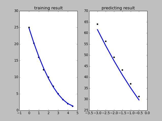
Figure: just right fitting demo
Overfitting demoWe use the polynominal to fit the data set.
$y = \theta _{0} + \theta _{1}x + \theta _{2}x^{2} + \theta _{3}x^{3} + \theta _{4}x^{4} + \theta_{5}x^{5} + \theta_{6}x^{6} + \theta_{7}x^{7} + \theta_{8}x^{8}$
And the predicting error is very large.
1 2 3 4 5 6 7 8 9 10 11 12 13 14 15 16 17 18 19 20 21 22 23 24 25 26 27 28 29 30 31 32 33 34 35 36 37 38 39 40 41 42 43 44 45 46 47 48 49 | import matplotlib.pyplot as plt import numpy as np from sklearn import linear_model from sklearn.metrics import mean_squared_error, r2_score #just plot x values in range 0, 10 step 0.5 x = np.arange(0, 5, 0.5) #generate y values x^2-10x+25 with noise in range [1,2] #we just get the left area parabola y = np.power(x-5, 2)+np.random.randint(2, size=x.size) #use polynominal theta0+theta1x+theta2x^+theta3x^3++theta4x^4++theta5x^5++theta6x^6++theta7x^7++theta8x^8 x_train = np.array([np.ones(len(x)), x, np.power(x, 2), np.power(x, 3), np.power(x, 4), np.power(x, 5), np.power(x, 6), np.power(x, 7), np.power(x, 8)]).T y_train = (y[:, np.newaxis]) #generate test data xx = np.arange(-3, 0, 0.5) yy = np.power(xx-5, 2)+np.random.randint(3, size=xx.size) x_test = np.array([np.ones(len(xx)), xx, np.power(xx, 2), np.power(xx, 3), np.power(xx, 4), np.power(xx, 5), np.power(xx, 6), np.power(xx, 7), np.power(xx, 8)]).T y_test = yy[:, np.newaxis] # Create linear regression object regr = linear_model.LinearRegression() # Train the model using the training sets regr.fit(x_train, y_train) #plot training y_pred1 = regr.predict(x_train) plt.subplot(121) plt.title('training result') plt.scatter(x, y_train, color='black') plt.plot(x, y_pred1, color='blue', linewidth=3) # Make predictions using the testing set y_pred2 = regr.predict(x_test) plt.subplot(122) plt.title('predicting result') # Plot predicting plt.scatter(xx, y_test, color='black') plt.plot(xx, y_pred2, color='blue', linewidth=3) # The coefficients print('Coefficients: ', regr.coef_) # The mean squared error print("Mean squared error: %.2f" % mean_squared_error(y_test, y_pred2)) # Explained variance score: 1 is perfect prediction print('Variance score: %.2f' % r2_score(y_test, y_pred2)) plt.show() |

Figure: Overfitting demo
6.1 Model selectionLet 's reuse the example above. How to find the 'best' polynomial degree for your hypothesis? Following the method:
- Shuffle and break down our data set into the three sets:
+ Training set: 60%
+ Cross validation set: 20%
+ Test set: 20%
- For each polynomial degree, calculating three separate error values for the three different sets using the following method:
+ Optimize the cost function using the training set
+ Using the cross validation set to choose the polynomial degree d with the least error: $J_{cross}(\theta ) = \frac{1}{2m_{cross}}\sum_{1}^{m_{cross}}(h(x_{cross}^{(i)}) - y_{cross}^{(i)})^{^{2}}$
+ For chosen polynomial degree d, estimate the generalization error using the test set with: $J_{test}(\theta ) = \frac{1}{2m_{test}}\sum_{1}^{m_{test}}(h(x_{test}^{(i)}) - y_{test}^{(i)})^{^{2}}$
This way, the degree of the polynomial d has not been trained using the test set.
6.2 Regularization
Let 's take the example of overfitting above and using regularization to reduce the magnitude of parameters θj by penalizing it. So it means we will make $\theta _{3} \approx 0, \theta _{4} \approx 0$ and finally the hypothesis becomes similar to $y = \theta _{0} + \theta _{1}x + \theta_{2}x^{2}$
The new cost function was introduced:
$J(\theta ) = \frac{1}{2m}\left [ \sum_{i=1}^{m} (h(x^{(i)}) - y^{(i)^{2}}) + \lambda \sum_{j=1}^{n}\theta _{j}^{2} \right ]\\
\lambda : \text{ Regularization parameter}\\
\text{if }\lambda \text{ is very large }\theta _{j} (j=\overline{1,n}) \approx 0\\
h(x) = \theta _{0}\text{ results in underfitting}\\
\sum_{j=1}^{n}\theta _{j}^{2} = \frac{\lambda }{2m}\theta ^{T}\theta = \left \| \theta \right \|_{2}^{2}:\text{ }
l_{2}\text{ or 2 norm regularization}$
When training set size m increases the effect of regularization part $\frac{\lambda}{2m} \sum_{j=1}^{n}\theta _{j}^{2}$ decreases.
In order to optimize the cost function that using regularization we use gradient descent algorithm with a slightly different:
$\text{The algorithm repeats for every j until convergence \{}\\
\text{ }\theta _{0} = \theta _{0} - \frac{1}{m}\alpha \sum_{1}^{m}(h(x^{(i)}) - y^{(i)})x_{0}^{i}\\
\text{ }\theta _{j} = \theta _{j} - \frac{1}{m}\alpha \sum_{1}^{m}(h(x^{(i)}) - y^{(i)})x_{j}^{i} - \alpha \frac{\lambda }{m}\theta _{j}\\
\text{\}}$
If applying regularization the normal equation becoms:
$\theta = (X^{T}X + \lambda \begin{bmatrix}
0 & 0 & 0 & 0\\
0 & 1 & 0 & 0\\
0 & 0 & 1 & 0\\
. & . & . & .\\
\end{bmatrix})^{-1}X^{T}Y\\
\lambda \begin{bmatrix}
0 & 0 & 0 & 0\\
0 & 1 & 0 & 0\\
0 & 0 & 1 & 0\\
. & . & . & .\\
\end{bmatrix})^{-1} \in R^{(n+1)(n+1)}\\
(X^{T}X + \lambda \begin{bmatrix}
0 & 0 & 0 & 0\\
0 & 1 & 0 & 0\\
0 & 0 & 1 & 0\\
. & . & . & .\\
\end{bmatrix})^{-1} \text{ this term is invertable}$
The term above is invertable so when applying regularization we should apply normal equation for fast calculation.
Let 's make a demo that use a simple training set. Try to adjust lamda to see the changes of parameters. It is not easy to choose the alpha parameter and lamda for gradient descent. You can check the error difference between 2 methods to see. If lamda is small the difference is small but lamda large the diffrence is large but the common error is large in both cases.
Using normal equation:
1 2 3 4 5 6 7 8 9 10 11 12 13 14 15 16 17 18 19 20 21 22 23 24 25 26 27 28 29 30 31 32 33 34 35 36 37 38 39 40 41 | import numpy as np #for inverse matrix from numpy.linalg import pinv import matplotlib.pyplot as plt x = np.array([-0.99768, -0.69574, -0.40373, -0.10236, 0.22024, 0.47742, 0.82229]) m = len(x) #generate y values x^2-10x+25 y = np.array([2.0885, 1.1646, 0.3287, 0.46013, 0.44808, 0.10013, -0.32952]) #form matrix x and Y X = np.array([np.ones(len(x)), x, np.power(x, 2), np.power(x, 3), np.power(x, 4), np.power(x, 5)]).T Y = (y[:, np.newaxis]) one = np.identity(X.shape[1]) one[0,0] = 0 lamda = 2 #apply normal equation theta = pinv(X.T.dot(X) + lamda*one).dot(X.T).dot(Y) print(theta) y_pred = theta.T.dot(X.T) plt.scatter(x, y, color='black') plt.plot(x, y_pred[0,:], color='blue', linewidth=3) plt.show() |
1 2 3 4 5 6 7 8 9 10 11 12 13 14 15 16 17 18 19 20 21 22 23 24 25 26 27 28 29 30 31 32 33 34 35 36 37 38 39 40 41 42 43 44 45 46 47 48 49 50 51 52 53 54 55 56 57 58 | #we use polynominal h(x) = theta0*x0 + theta1*x1 + theta2*x2 + theta3*x3 import matplotlib.pyplot as plt import numpy as np plt.figure(1) #just plot x values in range 0, 10 step 0.5 x = np.array([-0.99768, -0.69574, -0.40373, -0.10236, 0.22024, 0.47742, 0.82229]) m = len(x) #generate y values x^2-10x+25 y = np.array([2.0885, 1.1646, 0.3287, 0.46013, 0.44808, 0.10013, -0.32952]) plt.scatter(x, y, marker=r'$\clubsuit$') plt.hold(True) #convert to vectors x_train = np.array([np.ones(len(x)), x, np.power(x, 2), np.power(x, 3), np.power(x, 4), np.power(x, 5)]) y_train = (y[:, np.newaxis]) #h = theta0*x0 + theta1*x1 + theta2*x2 (x0=1 and x2=x^2) theta = np.array(np.zeros((x_train.shape[0], 1))) i = 0 alpha = 0.001 lamda = 1 preJ = 0 while (True): i = i + 1 h = theta.T.dot(x_train) error = h.T - y_train J = (error.T.dot(error) + lamda*theta[1::,0].T.dot(theta[1::,0]))/2*m; print(J) if(preJ == 0): preJ = J if(preJ < J): break else: preJ = J tmp = alpha*x_train.dot(error)/m tmp2 = tmp[1::,0] - alpha*lamda*theta[1::,0]/m theta[0,0::] = theta[0,0::] - tmp[0,0::] theta[1::,0] = theta[1::,0] - tmp2 print(theta) y_pred = theta.T.dot(x_train) plt.plot(x, y_pred.T) plt.show() |


0 Comments