k-Means Clustering is a unsupervised machine learning algorithm. It is the simplest Clustering algorithm.
The k-means algorithm searches for a predetermined number of clusters within an unlabeled multidimensional dataset. The algorithm will look for:
• The "cluster center" is the arithmetic mean of all the points belonging to the cluster.
• Each point is closer to its own cluster center than to other cluster centers.
k-Means Algorithm using the expectation maximization algorithm:
1. Random initialization some cluster centers
2. Repeat until converged
a. Assign points to the nearest cluster center
b. Set the cluster centers to the mean

2. Practice
from sklearn.datasets.samples_generator import make_blobs
import numpy as np
import matplotlib.pyplot as plt
import seaborn as sns
sns.set()
from sklearn.cluster import KMeans
from sklearn.metrics import pairwise_distances_argmin
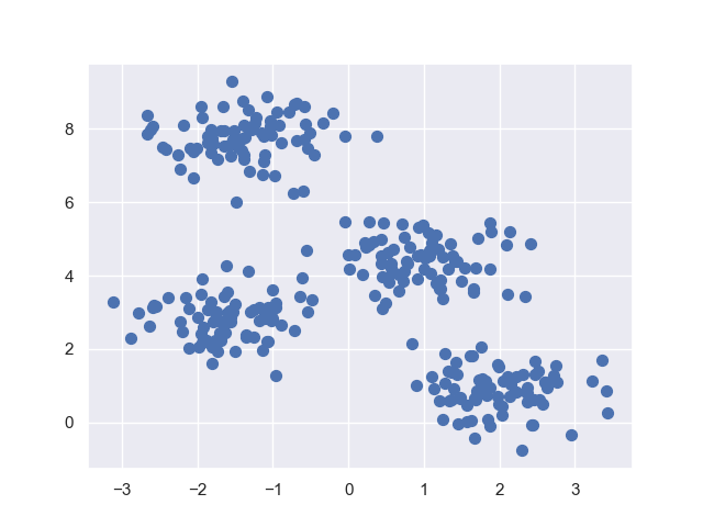
X, y_true = make_blobs(n_samples=300, centers=4, cluster_std=0.60, random_state=0)
#kmeans = KMeans(n_clusters=4,random_state=1)
#kmeans.fit(X)
#y_kmeans = kmeans.predict(X)
#plt.scatter(X[:, 0], X[:, 1], c=y_kmeans, s=50, cmap='viridis')
#centers = kmeans.cluster_centers_
#plt.scatter(centers[:, 0], centers[:, 1], c='black', s=200, alpha=0.5);
def find_clusters(X, n_clusters, rseed=2):
# 1. Randomly choose clusters
idx = np.random.choice(np.arange(X.shape[0]), n_clusters)
centers = X[idx]
while True:
# 2a. Assign labels based on closest center
labels = pairwise_distances_argmin(X, centers)
# 2b. Find new centers from means of points
new_centers = np.array([X[labels == i].mean(0) for i in range(n_clusters)])
# 2c. Check for convergence
if np.all(centers == new_centers):
break
centers = new_centers
return centers, labels
centers, labels = find_clusters(X, 4)
plt.scatter(X[:, 0], X[:, 1], c=labels, s=50, cmap='viridis');
plt.show()


Silhouette analysis can be used to study the separation distance between the resulting clusters. The silhouette plot displays a measure of how close each point in one cluster is to points in the neighboring clusters and thus provides a way to assess parameters like number of clusters visually. This measure has a range of [-1, 1].
Silhouette coefficients (as these values are referred to as) near +1 indicate that the sample is far away from the neighboring clusters. A value of 0 indicates that the sample is on or very close to the decision boundary between two neighboring clusters and negative values indicate that those samples might have been assigned to the wrong cluster.
from sklearn.datasets import make_blobs
from sklearn.cluster import KMeans
from sklearn.metrics import silhouette_samples, silhouette_score

import matplotlib.pyplot as plt
import matplotlib.cm as cm
import numpy as np

print(__doc__)

# Generating the sample data from make_blobs
# This particular setting has one distinct cluster and 3 clusters placed close
# together.
X, y = make_blobs(n_samples=300, centers=4, cluster_std=0.60, random_state=0)

range_n_clusters = [2, 3, 4, 5, 6]

for n_clusters in range_n_clusters:
    # Create a subplot with 1 row and 2 columns
    fig, (ax1, ax2) = plt.subplots(1, 2)
    fig.set_size_inches(18, 7)

    # The 1st subplot is the silhouette plot
    # The silhouette coefficient can range from -1, 1 but in this example all
    # lie within [-0.1, 1]
    ax1.set_xlim([-0.1, 1])
    # The (n_clusters+1)*10 is for inserting blank space between silhouette
    # plots of individual clusters, to demarcate them clearly.
    ax1.set_ylim([0, len(X) + (n_clusters + 1) * 10])

    # Initialize the clusterer with n_clusters value and a random generator
    # seed of 10 for reproducibility.
    clusterer = KMeans(n_clusters=n_clusters, random_state=10)
    cluster_labels = clusterer.fit_predict(X)

    # The silhouette_score gives the average value for all the samples.
    # This gives a perspective into the density and separation of the formed
    # clusters
    silhouette_avg = silhouette_score(X, cluster_labels)
    print("For n_clusters =", n_clusters,
          "The average silhouette_score is :", silhouette_avg)

    # Compute the silhouette scores for each sample
    sample_silhouette_values = silhouette_samples(X, cluster_labels)

    y_lower = 10
    for i in range(n_clusters):
        # Aggregate the silhouette scores for samples belonging to
        # cluster i, and sort them
        ith_cluster_silhouette_values = \
            sample_silhouette_values[cluster_labels == i]

        ith_cluster_silhouette_values.sort()

        size_cluster_i = ith_cluster_silhouette_values.shape[0]
        y_upper = y_lower + size_cluster_i

        color = cm.nipy_spectral(float(i) / n_clusters)
        ax1.fill_betweenx(np.arange(y_lower, y_upper),
                          0, ith_cluster_silhouette_values,
                          facecolor=color, edgecolor=color, alpha=0.7)

        # Label the silhouette plots with their cluster numbers at the middle
        ax1.text(-0.05, y_lower + 0.5 * size_cluster_i, str(i))

        # Compute the new y_lower for next plot
        y_lower = y_upper + 10  # 10 for the 0 samples

    ax1.set_title("The silhouette plot for the various clusters.")
    ax1.set_xlabel("The silhouette coefficient values")
    ax1.set_ylabel("Cluster label")

    # The vertical line for average silhouette score of all the values
    ax1.axvline(x=silhouette_avg, color="red", linestyle="--")

    ax1.set_yticks([])  # Clear the yaxis labels / ticks
    ax1.set_xticks([-0.1, 0, 0.2, 0.4, 0.6, 0.8, 1])

    # 2nd Plot showing the actual clusters formed
    colors = cm.nipy_spectral(cluster_labels.astype(float) / n_clusters)
    ax2.scatter(X[:, 0], X[:, 1], marker='.', s=30, lw=0, alpha=0.7,
                c=colors, edgecolor='k')

    # Labeling the clusters
    centers = clusterer.cluster_centers_
    # Draw white circles at cluster centers
    ax2.scatter(centers[:, 0], centers[:, 1], marker='o',
                c="white", alpha=1, s=200, edgecolor='k')

    for i, c in enumerate(centers):
        ax2.scatter(c[0], c[1], marker='$%d$' % i, alpha=1,
                    s=50, edgecolor='k')

    ax2.set_title("The visualization of the clustered data.")
    ax2.set_xlabel("Feature space for the 1st feature")
    ax2.set_ylabel("Feature space for the 2nd feature")

    plt.suptitle(("Silhouette analysis for KMeans clustering on sample data "
                  "with n_clusters = %d" % n_clusters),
                 fontsize=14, fontweight='bold')

plt.show()


0 Comments